Mutual Information is Copula Entropy

The paper
My experiments
Limitations
Appendix
Acknowledgement

This post is based on the paper Mutual Information is Copula Entropy by Jian Ma and Zengqi Sun.

The paper

The paper is on copula entropy. But before looking into it, let’s first define some basic concepts: entropy, mutual information and copula. For simplicity, let’s consider two random variables $X,Y$ .

Entropy. The entropy for $X$ is defined as

$\begin{equation*} H(X) = -\int p(X) \log p(X) \deriv X. \end{equation*}$

As this post will discuss copula entropy, to distinguish a few concepts later, I will also refer $H(X), H(Y)$ as the marginal entropy and $H(X,Y)$ as the joint entropy.

Mutual information. With these, we define the mutual information between $X$ and $Y$ as the difference between the sum of their marginals entropies and their joint entropy :

$\begin{equation*} I(X, Y) = H(X) + H(Y) - H(X, Y). \end{equation*}$

Copula. Finally, the Sklar theorem says that the joint distribution between $X,Y$ , $p(X,Y)$ , can be represented as a copula function $C$ with the help of cumulative distribution functions (CDFs) $F_X,F_Y$ as

$\begin{equation*} p(X, Y) = C(F_X(X), F_Y(Y)) \end{equation*}$

Note that $F_X(X), F_Y(Y) \sim \mathcal{U}(0, 1)$ . Intuitively speaking, the copula function $C$ contains and only contains all the dependency information between the random variables while the CDFs remove everything else.

Copula entropy. With these concepts being refreshed, we now define the copula entropy. For random variables $X,Y$ with uniform RVs from CDF transformations $U_X = F_X(X), U_Y = F_Y(Y)$ and the copula density $c(U_X, U_Y) \stackrel{\Delta}{=} \frac{\deriv ^2 C(U_X, U_Y)}{\deriv U_X \deriv U_Y}$ , the copula entropy is defined as

$\begin{equation*} H_c(X, Y) = - \int \int c(U_X, U_Y) \log c(U_X, U_Y) \deriv U_X \deriv U_Y. \end{equation*}$

With some massage (shown in their paper), one can show that

$\begin{equation*} I(X, Y) = -H_c(X, Y). \end{equation*}$

This appears to be interesting because the problem of estimating MI can be turned into first finding copula density function and then calculating the (negative) copula entropy. The authors argue that this is easier than estimating MI directly, which intuitively makes sense as $U_X,U_Y$ removes the complexity from the marginal. Notably, even $X,Y$ are in high dimensions, the estimation of copula entropy is always in the 2D space, although computing $F_X,F_Y$ in high dimensional space can be hard. The authors seem only consider univariate cases and suggest to do empirical copula density estimation based on sorting, which as far as I understand is a trick to computing the empirical CDFs efficiently (see later). For $N$ data points, the estimates are

$\begin{equation*} u_X^i = \frac{1}{N} \sum_{j=1}^N 1_{\{x^j \leq x^i\}} \quad\text{and}\quad u_Y^i = \frac{1}{N} \sum_{j=1}^N 1_{\{y^j \leq y^i\}}. \end{equation*}$

If the above is not yet clear to you, the MI estimation via copula entropy is simply two steps:

Computing $u_X^i,u_Y^i$ for $i=1,\dots,N$ from samples $\{x^i\}_{i=1}^N, \{y^i\}_{i=1}^N$
Using whatever entropy estimation method to estimate the entropy of samples $\{u^i\}_{i=1}^N$ where $u^i = \{u_X^i, u_Y^i\}$ (concatenation and yields RV in 2D).

Other than potential computational benefits, the relation between MI and copula entropy also leads to an interesting view of MI. The definition of copula entropy basically decouples marginal entropies and MI — you can have different marginal entropies and still get same MI or you can have the same marginal entropies but get a different MI due to different a copula function. Fig. 1 in their paper shows this observation nicely.

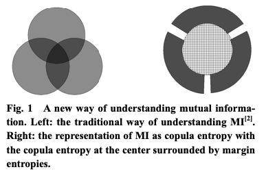
Figure 1: Fig. 1 from Ma and Sun (2011).

Another thing they show is that you can also write the joint entropy as a sum of marginal entropies and the copula entropy; see their paper for derivation:

$\begin{equation*} H(X, Y) = H(X) + H(Y) + H_c(X, Y). \end{equation*}$

It is an interesting view as copula entropy is the “entropy of their interrelations” while marginal entropy is entropy from marginals. In other words, this formulation decompose the sources of entropy. Again they have a nice figure showing this concept.

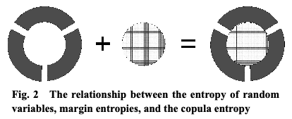
Figure 2: Fig. 2 from Ma and Sun (2011).

My experiments

The theory looks easy enough and I should be able to replicate their simulations on correlated Gaussians, that is, two Gaussians with covariance $\rho$ , for which the true MI is $-\frac{1}{2} \log (1 - \rho^2)$ . As a note, they use 1,000 samples from the Gaussians, compute the empirical inverse CDFs and use the Kraskov method to estimate the copula entropy. They compare their method against the true MI as well as some direct MI estimation method. They claim that the estimate is good while being much less computationally intensive.

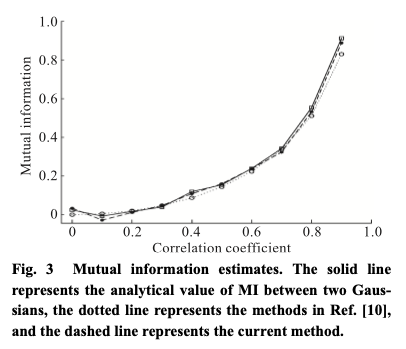
Figure 3: Fig. 3 from Ma and Sun (2011).

To compute $u = \{u_X, u_Y\}$ , I implemented the empirical estimate as stated in the paper in Julia (below). It has a complexity of $O(N^2)$ due to multiple calls of sum in the loop. There is a trick of making it $O(N \log N)$ by using sortperm, which I provide in the end of the post. But for now for clarity, let’s stick with this straightforward implementation.

function emp_u_of(x)
    u = zeros(length(x))
    for (i, xi) in enumerate(x)
        u[i] = sum(x .<= xi)
    end
    return u / length(x)
end

The empirical copula entropy can then be computed using some off-the-shelf entropy estimation method. Here I’m using the implementation of the Kraskov method available from Entropies.jl.

function emp_Hc_of(x, y)
    ux, uy = emp_u_of(x), emp_u_of(y)
    u = hcat(ux, uy)
    return genentropy(Dataset(u), Kraskov(k=3, w=0))
end

So how does this estimator perform? I follow up the setup in the paper but it doesn’t report the hyper-parameters ( $k,m$ ) of the Kraskov method they use. I didn’t tune the them either; I merely pick the default ones in the example of Entropies.jl but anyway here’s the plot that I reproduce. Looks not bad! Though it’s not as good as the one in the paper, probably because the entropy estimators are not exactly the same, it indeed confirms the relation between copula entropy and MI.

I also provide the MI estimate via estimating the 3 entropies in the definition of MI using the Krashov method directly, which actually turns out to be slightly better than the copula way.

Figure 4: MI via copula entropy with varied $\rho$ .

Limitations

One limitation I can see here is that the empirical CDFs can be hard to compute if the dimensionality of $X,Y$ is large. I go ahead to do the same toy experiment as in our TRE paper (Rhodes et al., 2020) by varying the dimension $d$ of two correlated Gaussians. I also show the copula entropy computed by the true CDF (using SciPy’s implementation). This can indicate the source of error of the overall estimate. Below are the results.

Figure 5: MI via copula entropy with varied $d$ .

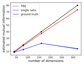
Figure 6: Figure 3 from Rhodes et al. (2020).

For reference, I also put the corresponding figure from Rhodes et al. (2020). Note the x-axes have different ranges. Also, I only use 10,000 samples for the copula approach (without true CDF) because otherwise the estimation is too slow, while our TRE paper uses 100,000 samples. For the copula approach with true CDF, I found 1,000 samples is enough to give good estimates and hence used here to make this plot.

Here I only plot the copula approach (green with crossings) for $2d\leq4$ , since a large $d$ leads to an estimate of negative infinity. This results from the poor empirical CDF estimation: it gives a constant vector of $u$ which then leads to a negative infinity entropy estimate. Even the copula density using the true CDF gives consistently biased estimates.¹ In short, even in this small region of $d$ , the estimator fails as $d$ goes larger. And even with the true CDF function, the estimator is biased. Are there any tweaks required to the estimation or this is just how badly it performs?

Note that to work with $d>1$ , we need to compute the multivariate CDF, whose empirical estimate for each $x^i$ is

$\begin{equation*} u^i = \frac{1}{N} \sum_{j=1}^N 1_{\{x_1^j \leq x_1^i, \dots, x_d^j \leq x_d^i\}} \end{equation*}$

My Julia implementation of it is below. Note that even I denote the estimate as $u$ , it’s NOT uniformly distributed as in the univariate case.

function emp_u_of(x::Matrix)
    d, n = size(x)
    u = zeros(n)
    for i in 1:n
        v = x .<= x[:,i]
        v = prod(v, dims=1)
        u[i] = sum(v)
    end
    return u / n
end

Appendix

Recall that emp_u_of in the main post has a complexity of $O(N^2)$ . A faster version of this univariate case that uses sortperm to achieve $O(N \log N)$ is shown below.

function emp_u_of_fast(x)
    u = zeros(length(x))
    sp = sortperm(x)
    for (i, j) in enumerate(sp)
        u[j] = i
    end
    return u / length(x)
end

You may also notice that the multivariate version of emp_u_of is “computationally inefficient” in the same sense. I didn’t see a clear way to do the same trick of using sortperm in this multivariate case.

Acknowledgement

Thanks Akash for proofreading the post and giving suggestions on the writing.

Footnotes:

: The two copula version do produce same values for $d$ smaller than or equal to 2.