A Short Note on Stratified Sampling

(Crude) Monte Carlo
- Example
Stratified sampling

Stratified sampling is a Monte Carlo (MC) method to estimate an integral that consist a distribution $p$ and a function of interest $f$

$\begin{equation*} I = \int_\sX p(x) f(x) \deriv x \end{equation*}$ 1

via partitioning $\sX$ into smaller groups, called strata. It is a type of quasi-Monte Carlo (QMC) method as it introduces deterministic procedures into the MC estimation. Same as crude Monte Carlo the estimation is still unbiased; however, the variance of the estimator can be smaller than crude MC.

(Crude) Monte Carlo

The (crude) Monte Carlo estimator of $I$ is

$\begin{equation*} \hat{I} = \frac{1}{N} \sum_{i=1}^N f(x^i) \end{equation*}$

where $x^i \sim p(x)$ and $N$ is the number of MC samples.

This estimator is an unbiased¹ estimator of the original target $I$ :

$\begin{equation*} \begin{aligned} \E[\hat{I}] &= \E \left[\frac{1}{N} \sum_{i=1}^N f(x^i) \right] \\ &= \frac{1}{N} \sum_{i=1}^N \E [f(x^i)] \\ &= \frac{1}{N} \sum_{i=1}^N I \\ &= I \end{aligned}. \end{equation*}$

Now let’s look at the variance of the estimator $\Var[\hat{I}]$ . We first need to define $\sigma^2 := \int_\sX p(x) (f(x) - I)^2 \deriv x$ , which is the variance of $f(x)$ under the distribution $p(x)$ . Now the variance of interest is

$\begin{equation*} \begin{aligned} \Var[\hat{I}] &= \Var \left[\frac{1}{N} \sum_{i=1}^N f(x^i) \right] \\ &= \frac{1}{N^2} \sum_{i=1}^N \Var[f(x^i)] \\ &= \frac{1}{N^2} \sum_{i=1}^N \sigma^2 \\ &= \frac{\sigma^2}{N} \\ \end{aligned}. \end{equation*}$

As it can be seen, the variance drops with the order of $O(\frac{1}{N})$ by using more samples.

Example

I now use an area estimation example² to demonstrate how the empirical estimate of the variance of the crude Monte Carlo estimator changes as the number of samples increases. The area $S$ I am interested in estimating is illustrated in the figure below.

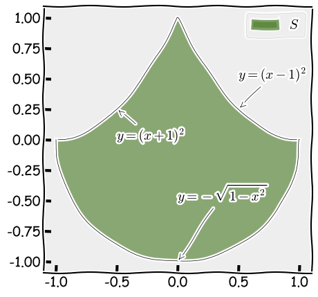
Figure 1: The area $S$

This is equivalent to computing the integral below

$\begin{equation*} \begin{aligned} S &= \int_{[-1, 1]^2} \1(x \in S) dx \\ &= 4 \int_{[-1, 1]^2} \frac{1}{4} \1(x \in S) dx \\ &= 4 \int_{[-1, 1]^2} \uniform(x; [-1, 1]^2) \1(x \in S) dx \end{aligned} \end{equation*}$

where $\1$ is the indicator function and $\uniform(x; \sA)$ is the uniform distribution over $\sA$ .

The crude MC estimator for $S$ is then

$\begin{equation*} \hat{S} = 4 \frac{1}{N} \sum_{i=1}^N \1(x^i \in S) \end{equation*}$

where $x^i \sim \uniform(x; [-1, 1]^2)$ and $N$ is the MC samples.

I now visualise how the variance of $\hat{S}$ changes as $N$ increases.

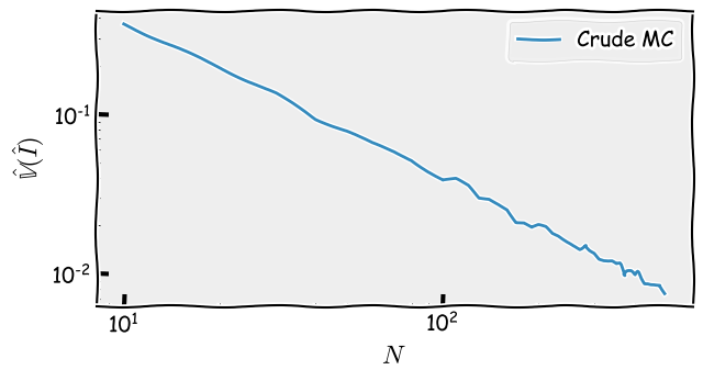
Figure 2: Variance convergence of crude MC

Note that both the x- and y-axis are in logarithm scale. As we can see, it matches our analysis results, which is $O(\frac{1}{N})$ .³

Stratified sampling

Now, we look at how stratified sampling works and how the variance of the corresponding estimator changes depending on different stratifications. For the sake of simplicity, we consider the case where $p(x) = \uniform([0, 1]^D)$ a $D$ -dimensional uniform distribution for the integral in equation 1.⁴ We first partition $\sX$ into $H$ strata s.t. $\sX = \sX_1 \cup \dots \cup \sX_H$ . Then, as the simplest way of performing stratified sampling, we uniformly draw independent Monte Carlo samples for each stratum $\sX_h$ , and the overall estimator is given as below

$\begin{equation*} \hat{I}_\text{strat} = \sum_{h=1}^H \frac{|\sX_h|}{n_h}\sum_{i=1}^{n_h} f(x_h^i) \end{equation*}$

where $\{x_h^i\}_{i=1}^{n_h}$ are samples that lie in $\sX_h$ and $n_h$ is the number of MC samples in stratum $h$ .

The mean of $f$ within each stratum $h$ is

$\begin{equation*} \begin{aligned} \mu_h &= \int_{\sX_h} \uniform(x; \sX_h) f(x) \deriv x \\ &= |\sX_h|^{-1} \int_{\sX_h} f(x) \deriv x \end{aligned} \end{equation*}$

and the corresponding variance is

$\begin{equation*} \begin{aligned} \sigma_h^2 &= \int_{\sX_h} \uniform(x; \sX_h) (f(x) - \mu_h)^2 \deriv x \\ &= |\sX_h|^{-1} \int_{\sX_h} (f(x) - \mu_h)^2 \deriv x \end{aligned}. \end{equation*}$

As it is mentioned in the beginning, $\hat{I}_\text{strat}$ is still an unbiased estimator of $I$ . We can validate this by computing the mean of $\hat{I}_\text{strat}$

$\begin{equation*} \begin{aligned} \E[\hat{I}_\text{strat}] &= \E\left[\sum_{h=1}^H \frac{|\sX_h|}{n_h}\sum_{i=1}^{n_h} f(x_h^i)\right] \\ &= \sum_{h=1}^H \frac{|\sX_h|}{n_h}\sum_{i=1}^{n_h} \E[f(x_h^i)] \\ &= \sum_{h=1}^H \frac{|\sX_h|}{n_h}\sum_{i=1}^{n_h} |\sX_h|^{-1} \int_{\sX_h} f(x) \deriv x \\ &= \sum_{h=1}^H \frac{1}{n_h}\sum_{i=1}^{n_h} \int_{\sX_h} f(x) \deriv x \\ &= \sum_{h=1}^H \int_{\sX_h} f(x) \deriv x \\ &= \int_{\sX_1 \cup \dots \cup \sX_H} f(x) \deriv x \\ &= \int_\sX f(x) \deriv x \\ &= I \end{aligned}. \end{equation*}$

The variance of $\hat{I}_\text{strat}$ is then

$\begin{equation*} \begin{aligned} \Var[\hat{I}_\text{strat}] &=\Var\left[\sum_{h=1}^H \frac{|\sX_h|}{n_h}\sum_{i=1}^{n_h} f(x_h^i)\right] \\ &=\sum_{h=1}^H \Var\left[\frac{|\sX_h|}{n_h}\sum_{i=1}^{n_h} f(x_h^i)\right] \\ &=\sum_{h=1}^H \frac{|\sX_h|^2}{n_h^2}\Var\left[\sum_{i=1}^{n_h} f(x_h^i)\right] \\ &=\sum_{h=1}^H \frac{|\sX_h|^2}{n_h^2}\sum_{i=1}^{n_h} \Var[f(x_h^i)] \\ &=\sum_{h=1}^H \frac{|\sX_h|^2}{n_h^2}\sum_{i=1}^{n_h} \sigma_h^2 \\ &=\sum_{h=1}^H \frac{|\calX_h|^2}{n_h}\sigma_h^2 \end{aligned}. \end{equation*}$

Effect of different allocation strategies

We are interested in comparing this estimator against (crude) Monte Carlo. In particular, we’d like to show that when $n_h$ is allocated proportionally to $|\sX_h|$ the estimator can only decrease in variance as compared to (crude) Monte Carlo.

In order to show this, we need to rewrite the variance of crude Monte Carlo in terms of strata. Let’s introduce $h(x)$ - the stratum that contains $x$ : $x \in \sX_{h(x)}, \forall x \in \sX$ . By the law of total variance, we have

$\begin{equation*} \begin{aligned} \sigma^2 = \Var[f(x)] &= \E[\Var[f(x) \given h(x)]] + \V[\E[f(x) \given h(x)]] \\ &= \sum_{h=1}^H |\sX_h| \sigma_h^2 + \sum_{h=1}^H |\sX_h| (\mu_h - I)^2 \end{aligned}. \end{equation*}$

Thus $\Var[\hat{I}] = \frac{\sigma^2}{n} = \frac{1}{n} \left( \sum_{h=1}^H |\sX_h| \sigma_h^2\right) + \frac{1}{n} \left(\sum_{h=1}^H |\sX_h| (\mu_h - I)^2 \right)$

Note that in the case of proportional allocation, because $n_h = n |\sX_h|$ ,

$\begin{equation*} \Var[\hat{I}_\mathrm{STRAT}] = \frac{1}{n} \sum_{h=1}^H |\sX_h| \sigma_h^2 \end{equation*}$

which is smaller than $\Var[\hat{I}]$ . Although it is not the optimal allocation⁵, proportional allocation as applied to stratified sampling will never increase the variance over that of crude Monte Carlo. Also, note that a poor allocation can also increase the variance of the estimator in comparison to crude Monte Carlo.

Effect of different stratification methods

It is interesting to note that, if $f$ is in 2D and is dominated by the horizontal direction more than the vertical direction, partitioning in the horizontal direction would be more effective than partitioning in the vertical direction. We will see it in the example soon.

Example (continued)

We continue with the example above by looking at 2 ways of stratifying the previously defined area.

Vertically partitioning the space into 10 parts
Horizontally partitioning the space into 10 parts

We illustrate where the samples are located for each method and for crude Monte Carlo in the figure below.

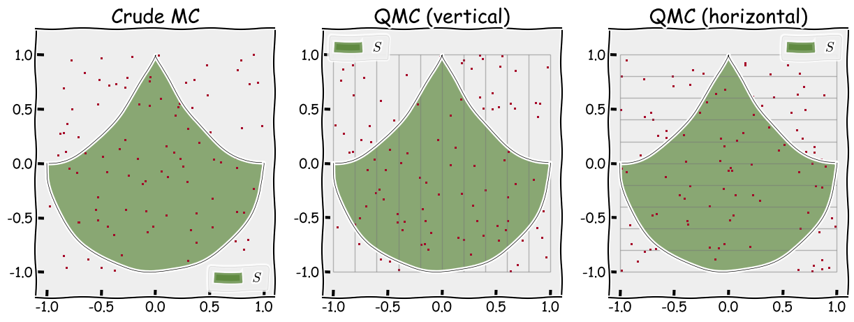
Figure 3: Different ways of sampling: crude MC (left), stratified sampling with vertical partitioning (middle) and stratified sampling with horizontal paritioning (right)

Notice that there are 100 samples in total for each method and that, for the stratified sampling methods, there are exactly 10 samples in each box.

Now what is interesting is the rate of variance of each estimator as the number of samples increase (shown below).

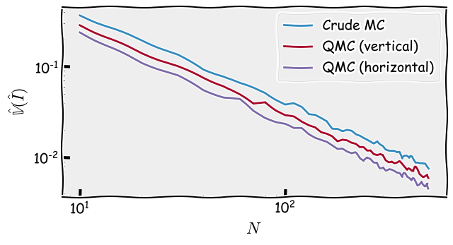
Figure 4: Variance convergence: crude MC v.s. quasi MC with different paritioning

As it can be seen, both QMC methods converge faster than crude Monte Carlo, as expected by our analysis. What’s more interesting is that horizontally partitioning the space is more effective than vertically partitioning it. This is because the pre-defined shape is dominated by the y-axis and not the x-axis. This domination can be explained by the shape’s symmetry along the y-axis and not the x-axis which means that the y-axis contains more information about the shape.